
Stop copying your data into other applications. Analyze your data right in Excel.
Stop copying your data into other applications. Analyze your data right in Excel.
Data too big for Excel? No problem, we can analyze data sets from Kilobytes to Petabytes.
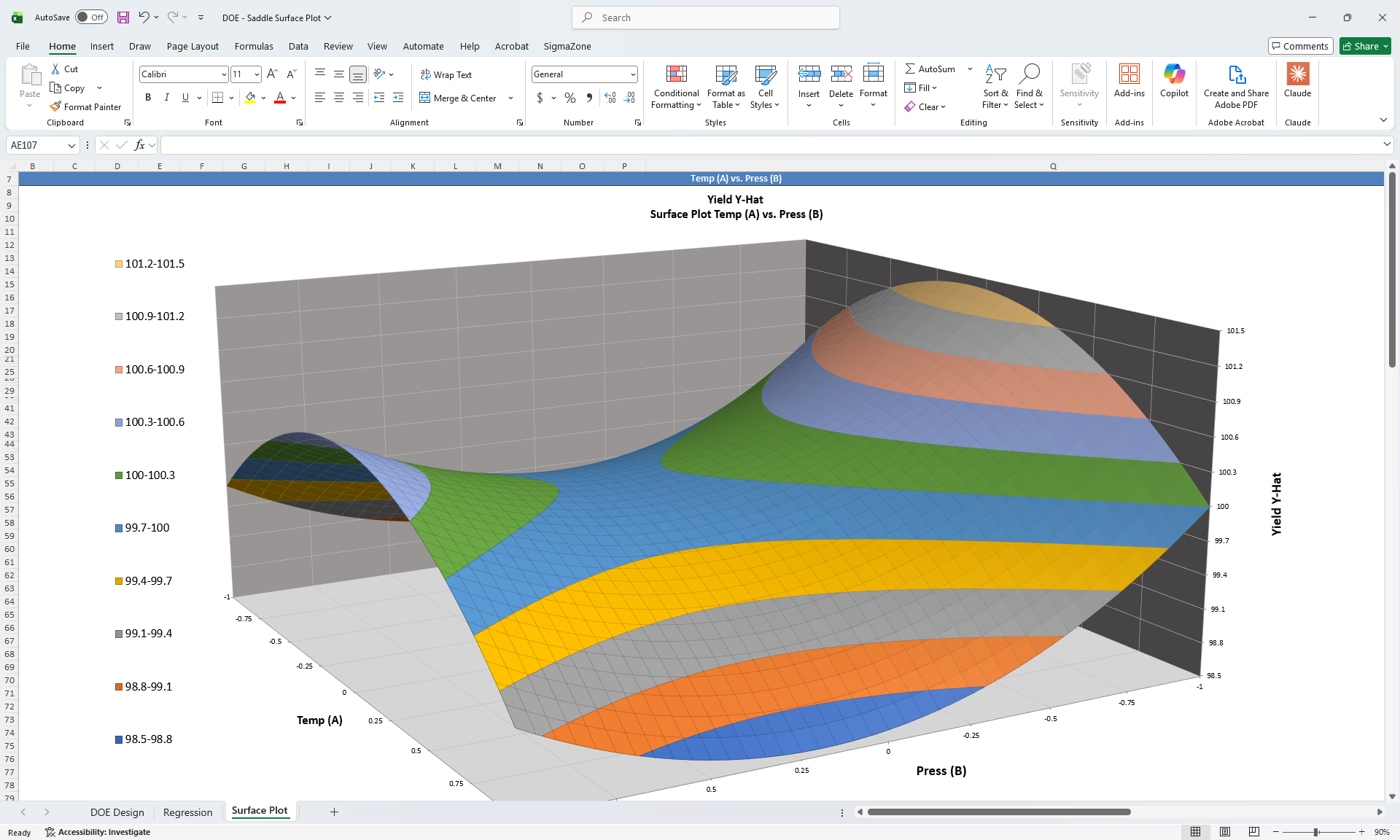
Statistical Tools, Design of Experiments (DOE), and Monte Carlo Simulation in Microsoft Excel.
Learn MoreStatistical simulations in Windows designed to help you practice your skills.
Learn More