Our Lens Simulator can be used to practice a number of statistical concepts including Cpk/Ppk analysis, control charts, hypothesis testing, and others. In this article I will show you how to do a simple t-Test and F-Test using Quantum XL using data from the simulator. If the simulator’s use isn’t obvious then go to this link for a 30 second video on how to use the simulator. The goal of the simulator is drag the lens to the center of the printed circuit board (PCB) while it is moving horizontally. The key metric is “Location Error” which is calculated as the distance from the center of the PCB to the center of the lens. If the lens is left/right of the center then the location error is negative/positive respectively. Below are three examples of location error. The ideal location error is equal to zero and the LSL = -20 mm with the USL = 20 mm, although the spec limits are not required to perform the t/F Test.
Location Error = -41 mm
Location Error = 0 mm
Location Error = +15 mm
When making the simulator, one of our developers made the suggestion to add a center line to the PCB to make it “easier” for the user. This erupted in a short but interesting debate as to the influence of the center line on location error which lead to this article. Thus, the objective of this experiment is to test the hypothesis that the center line on the PCB affects the mean and/or variance of the location error. To assist, we modified the simulator so the center line can be turned on and off using the “Toggle Center” button in the lower left corner of the simulation.
With Center
With Center
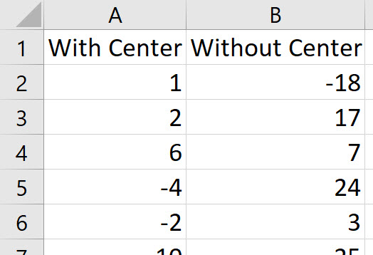
Using the simulator, I placed the lens 30 times without the center and 30 times with the center. I copied them into this Excel workbook. Quantum XL can analyze data in two different formats and are shown below. On the left is “Excel” format in which each data set is in a different column. On the right is “Group By” format is which all datasets are in the same column (see Location Error) but another column is used to delineate the data sets (see Center Status). Usages of “Excel” vs “Group By” format is largely a personal preference and you can freely switch between formats. In my experience, most people naturally enter data in “Excel” format. Group by format is more useful when exporting data from a database. For the purposes of this article we will use Excel format.
“Excel” Format
Each data set is in a unique column
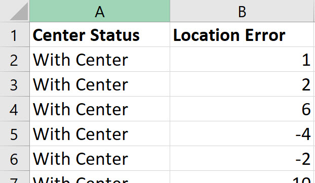
“Group By” Format
All data sets are in the same column (Location Error) with another column to identify the data sets (Center Status)
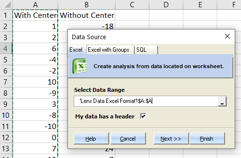
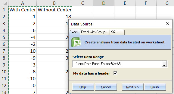
Before starting the t-Test or F-Test, the data should be checked for normality. Both the t-Test and the F-Test assume normality and so if the data isn’t normal a different test should be done. This article explains some of the other options. To run the Shapiro-Wilk test for normality in Quantum XL select “QXL Stat Tools” ribbon then “Hypothesis Test” > “Normality Test”. The data sets should be analyzed separately, so first select the data in column A. This can be most easily done by clicking on the column header (the A right above the words “With Center”). Your screen should look like this …
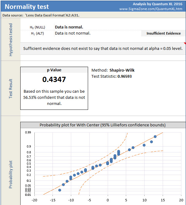
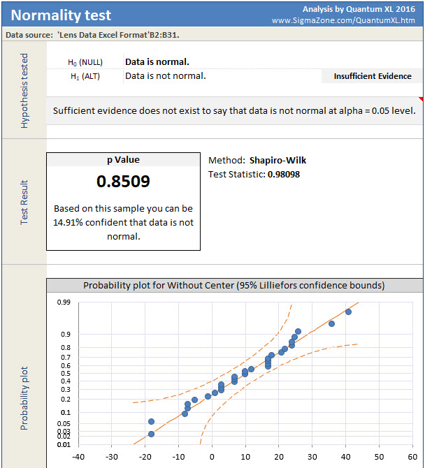
Quantum XL will display the results of the Shaprio-Wilk test as below. As the output indicates, there is insufficient evidence to reject normality at the alpha crit level = .05. At this point a statistician will warm up their lecturing voice and start to warn you that while we can’t reject normality we also can’t say that the data is normal. While this is of course correct, the average analyst doesn’t have the time or inclination to truly understand the nuance of how to interpret a p Value. If you would like to learn, then I would suggest articles by Cassie Kozyrkov who is Google’s Chief Decision Scientist. She has written numerous articles on the subject which handle this difficult concept better than most.
Since my sample size of n=30 isn’t too small and the Shapiro-Wilk test failed to reject normality, I’m going to assume the data is Normal. However, before I move on, I also need to check the data set in column B (without center).
Going through the same procedure, except this time choosing column B as the Data Range, we obtain the following. Again, given the fact that I have n=30 and fail to reject I’m going to assume that the data in column B (Without Center) is also normally distributed.
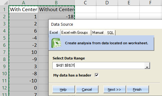
Before I move on, I should note that Quantum XL can run the Shapiro-Wilk test on multiple datasets at the same time. For example, I didn’t need to analyze Column A and B separately. To analyze them at the same time, simply start the process the same, i.e. select “QXL Stat Tools” ribbon then “Hypothesis Test” > “Normality Test”. Then select both columns A and B at the same time. See the “Select data Range” area below.
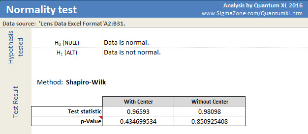
Which results in the analysis below. Note that the p-values are the same as the individual analysis.
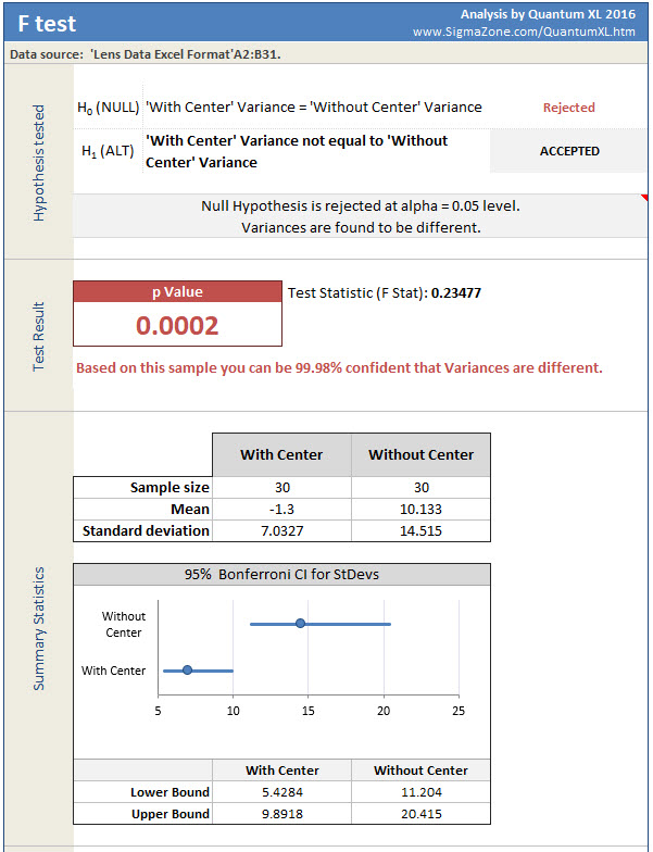
Now that I’m comfortable with the assumption of Normality, I’m ready to move onto the F-Test. The F-Test will test the hypothesis of equal variance. Specifically in this case, is the variation “With Center” the same or different than “Without Center”. It is important to test for equal variation before the t-Test as there are two different versions of the t-Test, one for equal variance and the other for unequal variance.
To start the F-Test in Quantum XL select “QXL Stat Tools” from the Excel ribbon then “Hypothesis Test” > “Test for Variation” > “F Test”.
The results of the F-Test are below. Of particular interest is the p-value which is .0002. At this point, I must be careful to avoid the wrath of the aforementioned statisticians. This is the way they would explain the p-value with a little clarification added by me. Imagine if you collected infinite samples from the simulator with and without the center displayed. If this infinite sample resulted in a stable distribution we can then refer to it as the “population”. From this population we took n=30 random samples from each population, that is population 1 “With Center” and population 2 “Without Center”. The standard deviation from my n=30 samples from “With Center” is equal to 7.0327. The standard deviation of my “Without Center” samples is equal to 20.415. If the population variances of “With Center” and “Without Center” were equal, we would expect to see this big of a difference in standard deviations in .0001 or .01% of the time. Since this is so unlikely, we can conclude the population variances are different with a very low probability of making a mistake.
While this is a correct definition, imagine trying to explain this to your boss or team or any other group that didn’t take the time to read this article. So, while this would make a lot of statisticians upset, I prefer the explanation “You can be 99.98% confident the variances are different”.
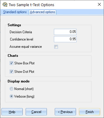
Now that we know that “With Center” and “Without Center” very likely have unequal variances, it is time to do the t-Test. There are two versions of the t-Test, one which assumes equal variance and the other which does not. By default, Quantum XL will use the equal variance t-Test but this is easy to change. Start the t-Test by selecting“QXL Stat Tools” from the Excel ribbon then “Hypothesis Test” > “Tests for Mean” > “Two Sample t-Test”. Just like in the F-Test, select both columns A and B. However, instead of clicking on Finish select “Next” which will bring you to the t-Test options. Click on “Advanced Options” and uncheck the box “Assume equal variance” (see below).
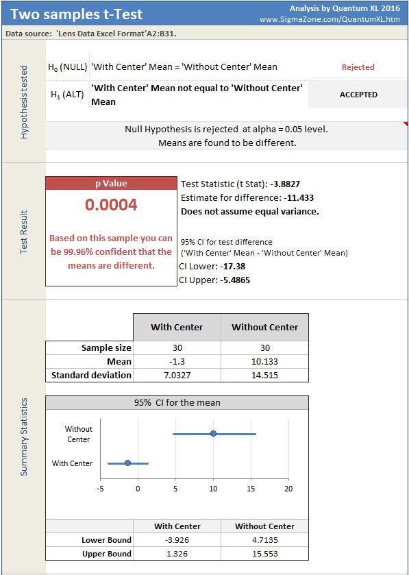
The results of the t-Test are below. The p-value is .0004 which the formal interpretation should be …
Imagine if you collected infinite samples from the simulator with and without the center displayed. This infinite sample would be the population data set. From this we took n=30 random samples from each population. The mean from my n=30 sample from “With Center” is equal to -1.3 mm. The mean of my “Without Center” sample is equal to 10.133 mm. If the population variances of “With Center” and “Without Center” were equal, we would expect to see this big of a difference in sample means in .0004 or .04% of the time. This is very unlikely so I will conclude the means are different.
However, an easier interpretation is that we are 99.96% confident the means are different. Based on this, we are very confident that my performance in placing the lens is closer to the center when a the center line is in place. A few other interesting observations from the data. Note that the mean location error for “Without Center” is equal to 10.133. This indicates my average error is 10.133 mm to the right of center (recall positive error is to the right of center and negative is to the left). The 95% confidence interval of the mean for “Without Center” is from 4.7135 to 15.553. Since this interval does not include zero, we are greater than 95% confident that I am biased to the right side of the target when placing the lens. The 95% confidence interval for the mean for “With Center” goes from -3.926 to 1.326 which does include zero. Therefore, I may tend to place the lens to the left or right, we don’t know yet. If I have a bias for left vs right when using the center target, it would take more samples to determine that.