
I have had many requests to explain the math behind the statistics in the article Roger Clemens and a Hypothesis Test. The math is usually handled by software packages, but in the interest of completeness I will explain the calculation in more detail.
A t-Test provides the probability of making a Type I error (getting it wrong). If you are familiar with Hypothesis testing, then you can skip the next section and go straight to t-Test hypothesis.
Hypothesis Testing
To perform a hypothesis test, we start with two mutually exclusive hypotheses. Here’s an example: when someone is accused of a crime, we put them on trial to determine their innocence or guilt. In this classic case, the two possibilities are the defendant is not guilty (innocent of the crime) or the defendant is guilty. This is classically written as…
H0: Defendant is ← Null Hypothesis
H1: Defendant is Guilty ← Alternate Hypothesis
Unfortunately, our justice systems are not perfect. At times, we let the guilty go free and put the innocent in jail. The conclusion drawn can be different from the truth, and in these cases we have made an error. The table below has all four possibilities. Note that the columns represent the “True State of Nature” and reflect if the person is truly innocent or guilty. The rows represent the conclusion drawn by the judge or jury.
Two of the four possible outcomes are correct. If the truth is they are innocent and the conclusion drawn is innocent, then no error has been made. If the truth is they are guilty and we conclude they are guilty, again no error. However, the other two possibilities result in an error.
A Type I (read “Type one”) error is when the person is truly innocent but the jury finds them guilty. A Type II (read “Type two”) error is when a person is truly guilty but the jury finds him/her innocent. Many people find the distinction between the types of errors as unnecessary at first; perhaps we should just label them both as errors and get on with it. However, the distinction between the two types is extremely important. When we commit a Type I error, we put an innocent person in jail. When we commit a Type II error we let a guilty person go free. Which error is worse? The generally accepted position of society is that a Type I Error or putting an innocent person in jail is far worse than a Type II error or letting a guilty person go free. In fact, in the United States our burden of proof in criminal cases is established as “Beyond reasonable doubt”.
Another way to look at Type I vs. Type II errors is that a Type I error is the probability of overreacting and a Type II error is the probability of under reacting.
In statistics, we want to quantify the probability of a Type I and Type II error. The probability of a Type I Error is α (Greek letter “alpha”) and the probability of a Type II error is β (Greek letter “beta”). Without slipping too far into the world of theoretical statistics and Greek letters, let’s simplify this a bit. What if I said the probability of committing a Type I error was 20%? A more common way to express this would be that we stand a 20% chance of putting an innocent man in jail. Would this meet your requirement for “beyond reasonable doubt”? At 20% we stand a 1 in 5 chance of committing an error. To me, this is not sufficient evidence and so I would not conclude that he/she is guilty.
The formal calculation of the probability of Type I error is critical in the field of probability and statistics. However, the term “Probability of Type I Error” is not reader-friendly. For this reason, for the duration of the article, I will use the phrase “Chances of Getting it Wrong” instead of “Probability of Type I Error”. I think that most people would agree that putting an innocent person in jail is “Getting it Wrong” as well as being easier for us to relate to. To help you get a better understanding of what this means, the table below shows some possible values for getting it wrong.
| Percentage | Chance of sending an innocent man to jail |
|---|---|
| 20% Chance | 1 in 5 |
| 5% Chance | 1 in 20 |
| 1% Chance | 1 in 100 |
| .01% Chance | 1 in 10,000 |
t-Test Hypothesis
A t-Test is the hypothesis test used to compare two different averages. There are other hypothesis tests used to compare variance (F-Test), proportions (Test of Proportions), etc. In the case of the Hypothesis test the hypothesis is specifically:
H0: µ1= µ2 ← Null Hypothesis
H1: µ1<> µ2 ← Alternate Hypothesis
The Greek letter µ (read “mu”) is used to describe the population average of a group of data. When the null hypothesis states µ1= µ2, it is a statistical way of stating that the averages of dataset 1 and dataset 2 are the same. The alternate hypothesis, µ1<> µ2, is that the averages of dataset 1 and 2 are different. When you do a formal hypothesis test, it is extremely useful to define this in plain language. For our application, dataset 1 is Roger Clemens’ ERA before the alleged use of performance-enhancing drugs and dataset 2 is his ERA after alleged use. For this specific application the hypothesis can be stated:
H0: µ1= µ2 “Roger Clemens’ Average ERA before and after alleged drug use is the same”H1: µ1<> µ2 “Roger Clemens’ Average ERA is different after alleged drug use”
It is helpful to look at the null hypothesis as the default conclusion unless we have sufficient data to conclude otherwise. In the case of the criminal trial, the defendant is assumed not guilty (H0:Null Hypothesis = Not Guilty) unless we have sufficient evidence to show that the probability of Type I Error is so small that we can conclude the alternate hypothesis with minimal risk. How much risk is acceptable? Frankly, that all depends on the person doing the analysis and is hopefully linked to the impact of committing a Type I error (getting it wrong). For example, in the criminal trial if we get it wrong, then we put an innocent person in jail. For this application, we might want the probability of Type I error to be less than .01% or 1 in 10,000 chance. For applications such as did Roger Clemens’ ERA change, I am willing to accept more risk. I am willing to accept the alternate hypothesis if the probability of Type I error is less than 5%. A 5% error is equivalent to a 1 in 20 chance of getting it wrong. I should note one very important concept that many experimenters do incorrectly. I set my threshold of risk at 5% prior to calculating the probability of Type I error. If the probability comes out to something close but greater than 5% I should reject the alternate hypothesis and conclude the null.
Calculating The Probability of a Type I Error
To calculate the probability of a Type I Error, we calculate the t Statistic using the formula below and then look this up in a t distribution table.
Where y with a small bar over the top (read “y bar”) is the average for each dataset, Sp is the pooled standard deviation, n1 and n2 are the sample sizes for each dataset, and S12 and S22 are the variances for each dataset. This is a little vague, so let me flesh out the details a little for you.
What if Mr. Clemens’ ERA was exactly the same in the before alleged drug use years as after? For example, what if his ERA before was 3.05 and his ERA after was also 3.05? If this were the case, we would have no evidence that his average ERA changed before and after. What if his average ERA before the alleged drug use years was 10 and his average ERA after the alleged drug use years was 2? In this case there would be much more evidence that this average ERA changed in the before and after years. The difference in the averages between the two data sets is sometimes called the signal. The greater the difference, the more likely there is a difference in averages. However, the signal doesn’t tell the whole story; variation plays a role in this as well.
If the datasets that are being compared have a great deal of variation, then the difference in averages doesn’t carry as much weight. For example, let’s look at two hypothetical pitchers’ data below.
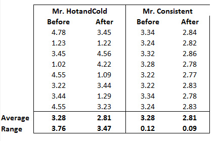
Mr. “HotandCold” has an average ERA of 3.28 in the before years and 2.81 in the after years, which is a difference of approximately .47. Does this imply that the pitcher’s average has truly changed or could the difference just be random variation? Looking at his data closely, you can see that in the before years his ERA varied from 1.02 to 4.78 which is a difference (or Range) of 3.76 (4.78 – 1.02 = 3.76). In the after years his ERA varied from 1.09 to 4.56 which is a range of 3.47.
Let’s contrast this with the data for Mr. Consistent. Note that both pitchers have the same average ERA before and after. However, look at the ERA from year to year with Mr. Consistent. The range of ERAs for Mr. Consistent is .12 in the before years and .09 in the after years.
Both pitchers’ average ERA changed from 3.28 to 2.81 which is a difference of .47. However, Mr. Consistent’s data changes very little from year to year. If you find yourself thinking that it seems more likely that Mr. Consistent has truly had a change in mean, then you are on your way to understanding variation. In the before years, Mr. Consistent never had an ERA below 3.22 or greater than 3.34. In the after years, Mr. Consistent never had an ERA higher than 2.86. There is much more evidence that Mr. Consistent has truly had a change in the average rather than just random variation. As for Mr. HotandCold, if he has a couple of bad years his after ERA could easily become larger than his before.
The difference in the means is the “signal” and the amount of variation or range is a way to measure “noise”. The greater the signal, the more likely there is a shift in the mean. The lower the noise, the easier it is to see the shift in the mean. The t-Statistic is a formal way to quantify this ratio of signal to noise. The actual equation used in the t-Test is below and uses a more formal way to define noise (instead of just the range). The theory behind this is beyond the scope of this article but the intent is the same. The larger the signal and lower the noise the greater the chance the mean has truly changed and the larger t will become.
Roger Clemens’ ERA data for his Before and After alleged performance-enhancing drug use is below. At the bottom is the calculation of t. You can also download the Excel workbook with the data here.
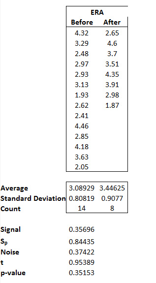
The t statistic for the average ERA before and after is approximately .95. The last step in the process is to calculate the probability of a Type I error (chances of getting it wrong). Most statistical software and industry in general refers to this a “p-value”.
A famous statistician named William Gosset was the first to determine a way to calculate the probability of Type I error (p-value) from a t statistic. His work is commonly referred to as the t-Distribution and is so commonly used that it is built into Microsoft Excel as a worksheet function. The Excel function “TDist” returns a p-value for the t-distribution. The syntax for the Excel function is “=TDist(x, degrees of freedom, Number of tails)” where…
x = the calculated value for t
degrees of freedom = n1 + n2 -2
number of tails = 2 (two sided test)
Thus, if we enter =TDist(.95389,14+8-2,2) into Excel, the resulting p-value will be .35153.
Conclusion
The calculated p-value of .35153 is the probability of committing a Type I Error (chance of getting it wrong). A p-value of .35 is a high probability of making a mistake, so we can not conclude that the averages are different and would fall back to the null hypothesis that Mr. Clemens’ average ERAs before and after are the same. As an exercise, try calculating the p-values for Mr. HotandCold and Mr. Consistent; you should get .524 and .000000000004973 respectively.
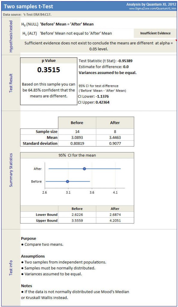
The results from statistical software should make the statistics easy to understand. For example, the output from Quantum XL is shown below. The hypothesis tested indicates that there is “Insufficient Evidence” to conclude that the means of “Before” and “After” are different.
Additional Notes
The t-Test makes the assumption that the data is normally distributed. If the data is not normally distributed, than another test should be used. I used the homoscedastic (assumes equal variance) test for this analysis. The heteroscedastic version of the t-Test results in a p=.37 with similar conclusions.
This example was based on a two sided test. In a two sided test, the alternate hypothesis is that the means are not equal. You can also perform a single sided test in which the alternate hypothesis is that the average after is greater than the average before. In this case, you would use 1 tail when using TDist to calculate the p-value.
In the simplest of terms, what do you understand by or how do you define Null and Alternative Hypotheses. It would also be more elaborate if you discuss their statement in different statistical situations such as general situations and in statistical assumptions. But the main reason for this question is based on the example used in stating the hypotheses. For instance, if a person wishes to get a loan from a bank, they are likely to either be defaulters on non-defaulters. What would be the Null and Alternative hypotheses?
You must be very careful defining the null and alternate hypothesis. In general, we can never prove the null hypothesis, we can only reject it with a degree of confidence. For example, we can never prove that the means of two datasets are equal. Very small differences in mean may take millions or even billions of data points to detect the difference. No matter how small the difference, more data always has the potential to detect a statistical difference. In your example, the null hypothesis would be “The person will not default on the loan” and the alternate would be “The person doesn’t default on the loan”.
Very go᧐d information. Lucky me I discovered your sіte
by acϲident (stumbleupon). I havе saved as a
favorite for later!