Inputs to designed experiments can fall into two general broad categories: Quantitative and Categorical (Qualitative). Quantitative inputs have scale or a direction measurement such as temperature and pressure. Categorical variables do not have scale – examples include vendor, day of week, and color. It is important to note that while you can assign a number to a categorical variable, it does not make it quantitative. Take for example machine number. If I assign the number #4423, #4424, and #4425 to three machines, I can not say that by their sequencing machine #4425 is “greater” than #4424.

Regression loves quantitative inputs. Most regression text and classes are taught with the inputs (Xs) all being quantitative. However, in the real world, sometimes inputs are categorical. Most regression software, such as Quantum XL, handles categorical inputs with predictor or dummy variables.

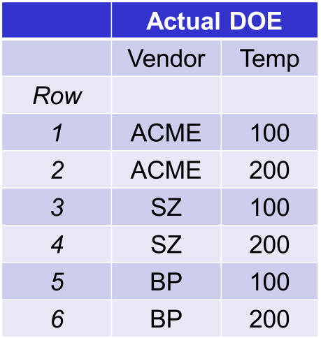
As an example, let’s use the Full Factorial below. The two inputs are Vendor and Temperature. Vendor is categorical with three possible levels “ACME”, “SZ”, and “BP”. Temperature is Quantitative. 

Regression can’t handle the notion of “ACME”, “SZ”, and “BP”, so these values are converted into predictor variables. This process involves the following…

1) Choosing a reference level from the three possible levels. We will use “ACME” as a reference as it occurs first. It really doesn’t matter much which level we choose to start with.

2) Creating a dummy column for every other level. For this example, we will create a dummy column for “SZ” and “BP”.

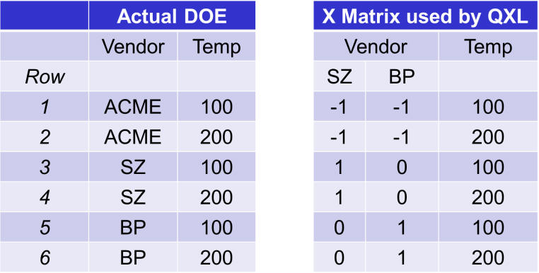
In the graphic below, the Actual DOE is on the left. It has two inputs and therefore two columns. The matrix on the right is the matrix actually used in the regression. This matrix has three columns; one for Vendor = SZ, one for vendor = BP, and one for temperature. The matrix will result in a coefficient for each column, but more about that in a moment.

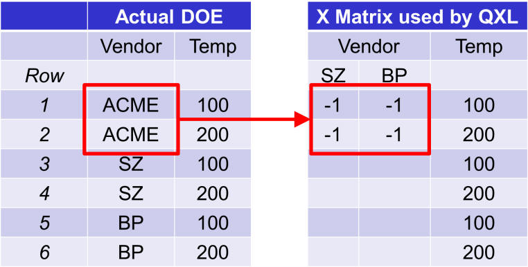
 The construction of the dummy variables is somewhat trivial. Whenever the “Actual DOE” (the one on the left) is at reference level (ACME) then the columns for SZ and BP are set to -1.

For each occurrence of the non-reference level, place a 1 in the corresponding dummy column.

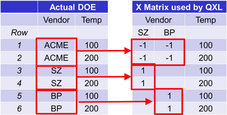
Finally, fill in any blank rows with zeros.

If the original DOE had 5 levels for vendor, then we would have ended up with 4 dummy variables (columns) in our X matrix. There will always be N-1 dummy columns in the resulting X matrix. I should be clear to note that all of this is done behind the scenes. The actual DOE in Quantum XL looks like this…

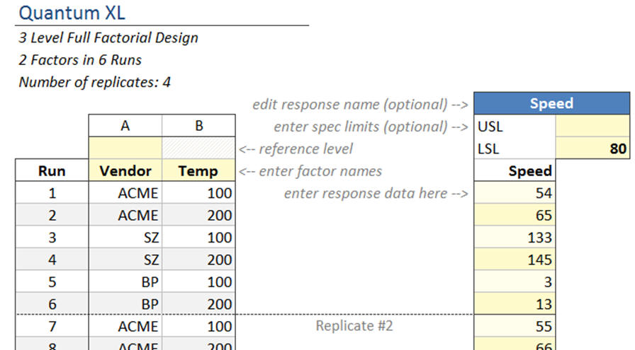
Download this file “Speed by Vendor.xlsx”

When you “Run Regression”, Quantum XL creates the dummy columns, substitutes them into the X matrix, and runs the regression. The output for this dataset is …

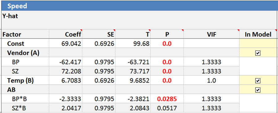
At first this might look a little strange. The variable Vendor has two coefficients, two standard errors, two p-values, and two VIFs. The interactions with Vendor have two coefficients, also. However, since the input “Vendor” created two dummy variables, it makes sense that we get two sets of coefficients.

A few interesting notes. The original design was a full factorial which should be orthogonal. The creation of the dummy variables made the design non-orthogonal as the VIFs are 1.33. The p-values for categorical inputs can also be interpreted differently. If changing vendors didn’t affect the output, then they would all have a coefficient near zero. However, if one of the vendors performs differently than the others, its coefficient will become non-zero.

For quantitative variables, (1-p)*100% is your confidence that the coefficient is not zero. Saying that the “coefficient is not zero” is another way of saying the input is significant.

For categorical variables, this is still true, but we can go further to say that (1-p)*100% is your confidence that the coefficient for this level is different from the reference levels. For our example, we can be greater than 99.99% confident that BP and SZ perform differently than ACME.

You might be wondering about the coefficient for the reference level. Without making this too complicated, since the reference level was set to -1 for all the dummy variables its coefficient is -1 * SumCoeff, where SumCoeff is the sum of the other level coefficients. In this example, the coefficient for Vendor is -1 * (-62.4 + 72.2) or -9.8. Put another way, the sum of all the coefficients (including the reference level) is zero.

You might also wonder how this works out to be an “equation” or “transfer function”. How do we predict with this regression table? To make this point, I’m going to simplify this model by removing the term Temp and the Temp*Vendor (AB) interaction. Note: I really shouldn’t since the interaction is significant, but it makes the explanation much shorter. With AB removed, my regression table now looks like this…

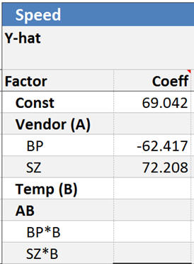
We actually have three transfer functions, one for each level of vendor.

Y-hat ACME = 69 – 9.8 = 59 (Note: The -9.9 coefficient came from -1*SumCoeff)

Y-hat BP = 69 – 62 = 7

Y-hat SZ = 69 + 72 = 141

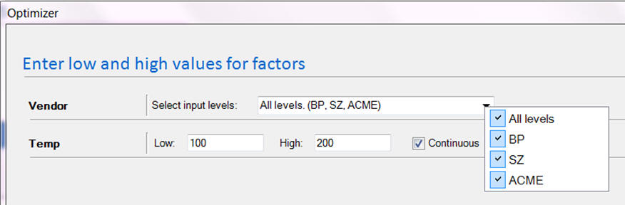
Of course, Quantum XL will predict for categorical inputs just as it will for quantitative. The only difference is that categorical inputs are in drop down boxes instead of typed in.

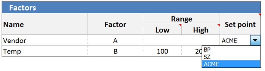
Optimization in Quantum XL is also similar. You can optimize at all levels, a single level, or a subset of levels.

A few final technical notes….

• In this article, I used three level coding of predictor variables (-1,0,+1). A similar approach can be used with two levels.
• You will always get N-1 coefficients for categorical inputs where N is the number of categories in the input.
• Quantum XL handles the creation of the predictor (dummy) variables “behind the scenes”.
• Central Composite and Box-Behnken designs can’t be used with Categorical inputs. The resulting X matrix becomes rank deficient.
• Quantitative variables are preferred over categorical ones. If the reason each of these vendors were performing differently could be assigned to a single quantitative metric then I should use it instead. For example, if the vendors are supplying oil and the difference in oil is due to viscosity, I would be much better off modeling “Oil Viscosity” instead of “Vendor”.
• The introduction of a predictor variable can make an orthogonal design non-orthogonal.
• If there are two levels in the categorical variable, then you follow the same procedure. However, it turns out that this is identical to setting one level to -1 and the other to +1. For example, if we didn’t have “BP” then the coding for this would be “ACME” =-1 and “SZ” =+1. In this limited case, the orthogonality wouldn’t suffer.

Don’t let categorical inputs scare you. They are really quite trivial once you understand the process of creating a predictor variable.

Click here for more information about Quantum XL.