
In this tutorial we will lead you through the process of setting up a DOE, analyzing it with regression/ graphical tools, and optimizing the output. This tutorial is not a replacement for DOE training, but rather an introduction to Quantum XL for those of you who have DOE experience.
- Step #1: Setting up the Designed Experiment
- Step #2: Analyzing the DOE using Regression, Interpreting the Results, and Predicting
- Step #3: Confirming the DOE with validation runs
- Step #4: Using the graphical tools
- Step #5: Optimization
Step #1: Setting up the Designed Experiment
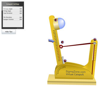
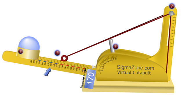
For this tutorial, we will be using the virtual catapult located at the link below. The catapult can be “shot” like a real catapult allowing the real-time collection of data. If you are a virtual pacifist or suffer post-traumatic stress disorder circa the middle ages, then you can skip the shooting and download a completed file. No bits or bytes were harmed in the making of this tutorial.
The virtual catapult is written in Microsoft Silverlight which is only compatible with Internet Explorer (not Microsoft Edge or Google Chrome).
Link: https://sigmazone.com/SL/Catapult/

To shoot the catapult, click and drag the arm back to the desired angle and then release the left mouse button.
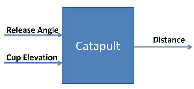
Our goal is to build a model for Distance as a function of Release Angle and Pin Elevation or Distance = f(Release Angle, Pin Elevation).
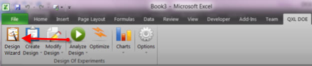
Our first step is to create the design. Quantum XL has a slew of experimental design choices. They can be found directly from the QXL DOE -> Create Design menu. However, remembering which DOE to use in each specific situation requires memory cells that you would probably rather commit to something else. To make things easy, we’ve put in a Design Wizard that will take you through the process step by step.
Click on the tab “QXL DOE” and then “Design Wizard” from the ribbon.
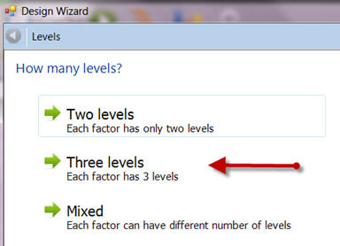
2-Level or 3-Level
Your first decision is to choose the number of levels in the design. In this case, we suspect that the distance the catapult will shoot (our output) will have curvature. To model curvature, we need a model with quadratics (A2, B2, …). Thus, we need a three-level DOE.
Click on “Three levels”
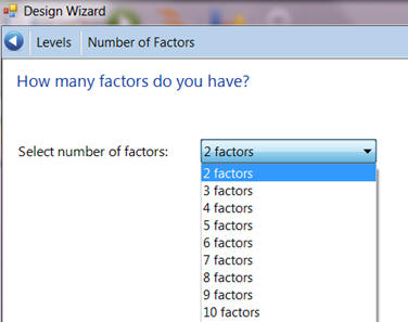
Number of Factors
The next piece of information is the number of factors in the design. Unfortunately, statisticians have felt the need create multiple synonyms for factors over the years. You may have heard them called “Inputs”, “Main effects”, “Factors”, “Terms”, “Variables”, or even “Independent Variables” by someone who is overly impressed with themselves.
Since we want to model both “Release Angle” and “Cup Elevation” we will select “2 factors” and then click “Next”.
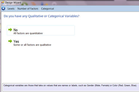
Categorical (Qualitative) Variables
Selecting the correct design is dependent on the type of inputs in your DOE. The types can be either Quantitative or Categorical. Again, we have the multi-name thing going on; categorical is the same as qualitative.
If you’ve never heard of either one, the pay attention to the tip at the bottom of the screen. It tells you that Categorical inputs are variables that take on levels such as Gender or Color. Variables with a direct measurement like temperature or pressure are quantitative.
Release Angle and Cup Elevation are both Quantitative, so click on “No, all factors are quantitative” to move on.
Choose a Design
Quantum XL will now show the designs that match your specific setup. In this case, there is only one; CCD or Central Composite Design. Quantum XL will display “Recommended” in red next to the design that is the best choice for your specific situation.
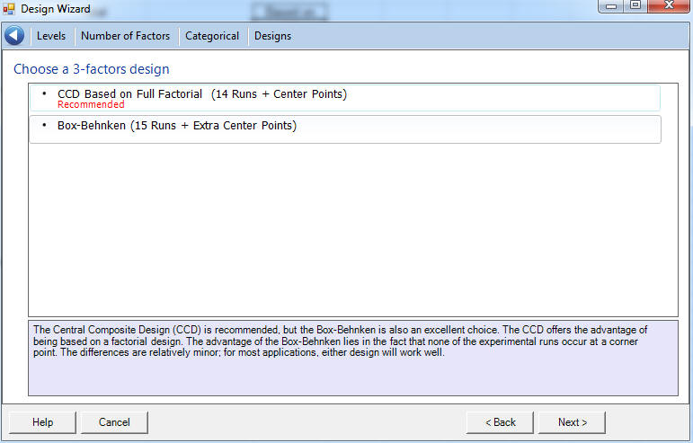
Click on “Next”
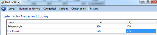
Enter Factor Names and Coding
While we could do the DOE with factor names “A” and “B”, it is much easier to use the actual names of the variables. Replace A with “Release Angle” and B with “Cup Elevation”. The low and high values are the range of experimentation. Replace the low/high for Release Angle to 150/170 and for Cup Elevation to 225/275.
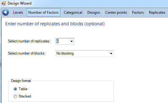
Replicates and Blocks
Replicates are repetitions of experiments to better estimate the variability in a model. Change the number of replicates to 4. Blocking is a slightly advanced method to isolate nuisance variables. We don’t have any nuisance variables, so leave the number of blocks to “No Blocking”.
The design format can be either “Table” or “Stacked”. When the design is in table format, the replicates are in adjacent columns. In stacked format, the replicates are arranged vertically in a single column. For most users, table format is easier to use. If you change your mind later, use the menu items under “Modify Design” to convert from table to stacked and vice versa.
Leave “Design format” set to “Table” and press “Finish”.
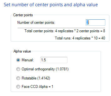
Center and Alpha Value
The CCD has some specific parameters that are not applicable to any other design. You need to choose the number of center points and the alpha value. Center points are repeated observations at the center of the design space. Change the number of center points to 2.
Since you’ve already chosen four replicates, Quantum XL points out that “4 replicates * 2 center points = 8” which means we will have 8 observations at the center value.
The alpha value can be either manual, optimal orthogonality, rotatable, or Face Center CCD. While an orthogonal or rotatable design is admirable, it is often hard to obtain. In our application, we’re going to use a value of 1.5, simply to make the axial values more visible. Change the Alpha Value “Manual” setting to 1.5 and click Next.
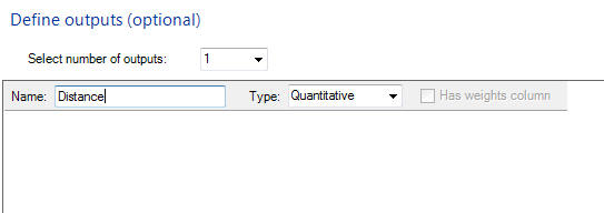
Define Outputs
Quantum XL can model multiple outputs (responses) simultaneously. In this step you can optionally increase the number of outputs and define their type (Quantitative, Binary, or Nominal). In our case, we have one output which is distance. Since the distance the ball travels is quantitative, we can leave the type to the default.
Change the name of the output to “Distance” and press Next.
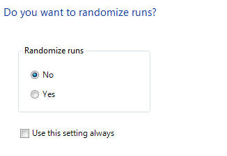
Randomization
Randomization of the run order is a good idea if time dependency is of concern. In our case, the simulator doesn’t have a time dependency so I have opted to not randomize. If you would like to randomize, feel free to select “Yes” and continue.
Select “No” for randomize runs and press “Finish”.
Collect and Enter Data
Quantum XL will now create a new worksheet entitled “DOE Design”. The sheet will include the design information in the upper left hand corner (i.e., Central Composite Design, Base Design: full factorial….).
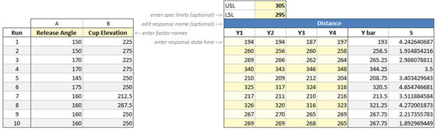
On the left hand side is the experimental design, in this case the CCD. On the right side is the area where you can enter the replicated data.
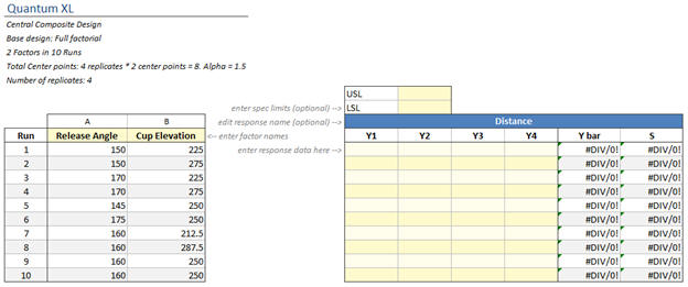
In light grey, you can see additional instructions. The first is to “enter spec limits”. While this is an optional step, if you have spec limits then enter them to have Quantum XL calculate predicted Cp, Cpk, and dpm.
Enter 295 for the LSL and 305 for the USL.
The second light grey instruction is to “edit response name”. We already named the output “Distance” while we were in the Design Wizard, but we could change it here if needed.
The third light grey instruction is to “enter factor names”. We also did this during the wizard, but they can be edited here. Finally, the last instruction is the enter response data.
It is time to collect our data. Go to the virtual catapult at this link https://sigmazone.com/SL/Catapult/ and start collecting your data.
Note that the catapult has more than two factors. The inputs firing angle, pin elevation, and bungee position should be left at their default settings.
The first row calls for a Release Angle = 150 and a Cup Elevation = 225. With your mouse, click and drag the “cup” to a height of 225.
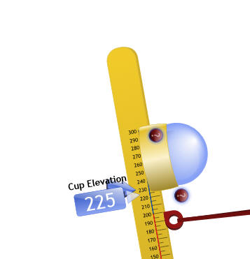
Then click and drag the arm back to an angle of 150.
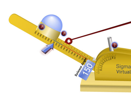
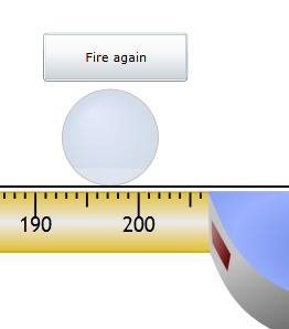
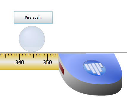
Release the mouse and the catapult will fire. When the ball lands, a tape measure will come out so you can collect the measurement.
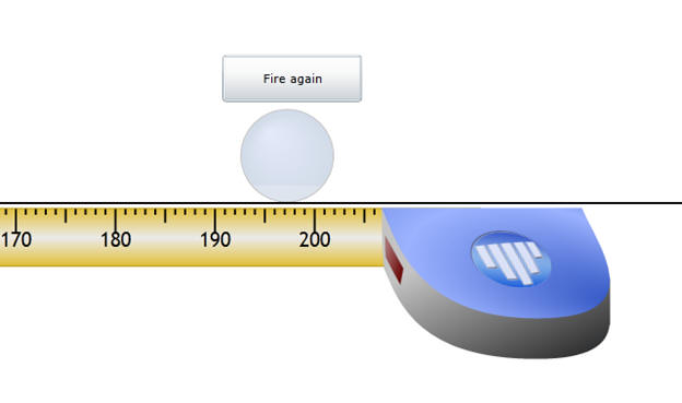
I am measuring to the center of the ball, which is 197 cm.
Enter this distance of your shot into the design sheet under “Y1”.
Note: The catapult has variation, your distance may be different than 197.
You have just collected the first of 40 data points. Press the “Fire again” button and collect the rest of the data.
If you don’t want to collect the 39 other data points, you can download a completed file from the link below. Keep in mind that you will be missing the opportunity to enjoy the exceptional work of our outstanding programmers, but don’t let that hold you back.
Download: Virtual Catapult DOE Completed.xlsx
Step #2: Analyzing the DOE using Regression, Interpreting the Results, and Predicting
Your design sheet should now have the data entered for the replicates. Again, the catapult has variation, so if you chose the noble path of collecting your own data, your numbers may be slightly different.
Since our output is Quantitative, the primary method of analysis is Ordinary Least Squares Regression. Most people just call this “Multiple Regression” or “Regression”. Quantum XL also supports Binary Logistic Regression for Binary output and Nominal Logistic Regression for Nominal Outputs. Luckily, you don’t have to remember any of that as Quantum XL will automatically use the correct type of regression for your model.
From the QXL DOE tab select “Analyze Design” -> “Run Regression”.
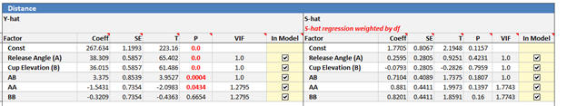
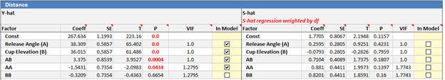
Quantum XL automatically models both Y-hat and S-hat (f enough data is available). The model on the left is Y-hat while the model on the right is S-hat.
Some competing software will model S-hat but make you jump through hoops in the process. A commonly asked question is “Where did Quantum XL get the data to model S-hat?” When you collected the data, you had multiple replicates for each run. This can be seen easily in the columns to the right of the replicates.
Just to the right of the four replicates are the columns “Y bar” and “S”. These are calculated values, each coming from the four replicates. Hence the first Y bar value (193) is the average of the first four replicates (194, 194, 187, and 197). The first “S” is the standard deviation of the first four points. Quantum XL creates a new response from the S column and models it at the same time. More information can be found in the section Modeling S-hat.
Why model S-hat?
A better question would be “Why not?” The mean is relatively easy to change; the standard deviation is much harder. If you can find an input that changes the standard deviation, then you’ve struck gold. Many of the S models will have no significant inputs. However, if yours does then you’ve just found a way to reduce the standard deviation. On the downside, your computer does have to do several million more calculations to bring you the S-hat model. You may have to wait a thousandth of a second longer for the results.
Warnings
Quantum XL will automatically check your model for a variety of “problems” that you might be interested in. If you are using my data, then you should have gotten a warning at the top of the regression table.

When you click on this red bar, Quantum XL will jump to the warnings section which clearly denotes any problems with the model. In my case, it turns out that the third replicate of the first run has a larger standardized residual than expected. To be fair, when I was collecting this data point, I was distracted by the football that my son had hurled at a concerning velocity on a trajectory which would collide with my head.
Points with larger standardized residuals are influential and may potentially be outliers. Many people would immediately delete or recollect this data… I consider this a mistake. If there is a valid reason (aka impending collision with football) that this point is not representative of the process, then I could safely remove this point. However, if not then the point is telling me I have more variation for this run.
Since there was only one potential outlier and it wasn’t very extreme, I opted to leave it in. Later, if I was to fail to validate, I might reconsider this decision.
The Statistics
For the purposes of this tutorial, we will assume that you already understand regression statistics. If you don’t, Quantum XL has “pop up” help for every stat on the regression table. For example, if you hover your mouse over the “P” the following tip will pop up until you move your mouse. For more information on statistics, see the section on Ordinary Least Squares.

Reducing the Model
Remove the check mark in the terms that aren’t significant. None of the terms in the S-hat model appear to be significant and we removed the BB (B2) term from the Y-hat model.
S-hat Model: Remove all the check marks “In Model”
Y-hat Model: Remove the check mark under BB “In Model” (see below)
Select “Analyze Design” – “Run Regression” from the QXL DOE tab to obtain the reduced model.
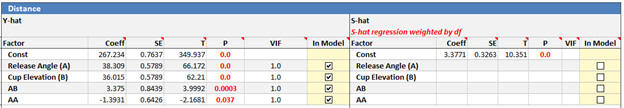
Now that you’ve got a reduced model, you can predict, graph, and optimize using the model.
Prediction
With Quantum XL prediction is a breeze. Just above the Y-hat regression table you’ll find the “Factors” and “Prediction” area. The prediction area calculates the Y-hat, S-hat, Prediction Interval, Cp, Cpk, and DPM for the values of the set points. The default set points are the center points or in this case Release Angle = 160 and Cup Elevation = 250.
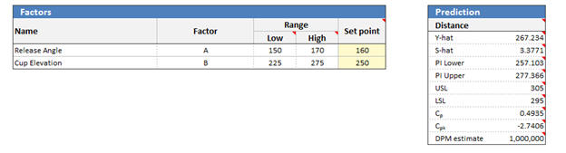
If we were interested in Release Angle = 170 and Cup Elevation = 275 then we simply type those values into the cell “Set Point”. The predicted distance (Y-hat) is now 343.54 cm, the predicted standard deviation (S-hat) is 3.3771. The Prediction Interval (PI) is from 333 to 353 cm. The prediction interval is the range in which you expect most of the validations runs to occur.
Step #3: Confirming the DOE with validation runs
To validate our model, we need to go back to the catapult and use these set points for the input. Drag the cup elevation to 275 and pull back to 170 degrees. Release the mouse… enjoy watching the virtual tiny blue ball flying through the frictionless air until it comes to rest and waits anxiously for you to measure it.
The ball should travel between 333 cm and 353 cm. In this case, the ball did; it traveled 344 cm.
If the ball fell outside this range, then the model would have failed to validate. Checking one point isn’t sufficient, so I ran a total of 10 validation runs. The 10 shots were 344, 343, 345, 347, 341, 346, 340, 342, 338, and 342. All 10 of these runs fell within the prediction interval of 333 cm to 353 cm. Note: This really isn’t a great place to validate our model. We collected data at Release Angle = 170 and Cup Elevation = 275, so we would expect the model to work well here. A better place would be either at our optimal or a point in which we’ve never collected data.
Step #4: Using the graphical tools
Quantum XL can create a myriad of graphs. The most basic is the Pareto of regression coefficients. Select “Graphs” then “Pareto of Regression Coefficients” from the QXL DOE tab. The next screen allows you to display the Pareto for Y-hat, S-hat or Both, as well as change the number and orientation of the bars. In this case, leave everything at the default and press “Create and Exit”.
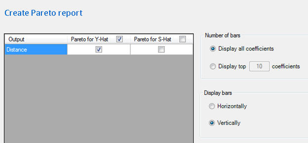
The resulting Pareto provides a graphical representation of the strength of each term. The term with the greatest impact on the model is Release Angle followed by Cup Elevation.
Interactions Plots
To create an interaction plot, go back to a regression table and select “Charts” -> “Interaction Plots” from the QXL DOE tab. Note: if you aren’t on a regression table when you start making a chart, Quantum XL will ask you which regression table to use. From here you can chose which terms to plot. For more information, see the interaction plots topic in the help system. We’ll leave the default and click on “Create and Exit”.
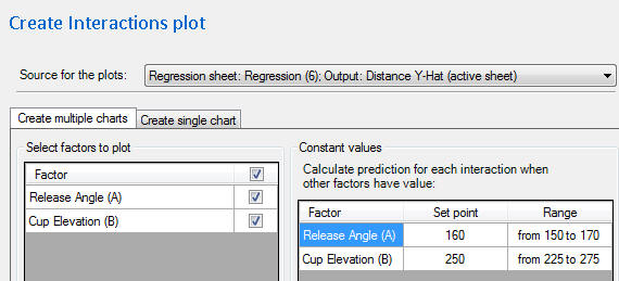
Quantum XL will create the chart using the levels used in the DOE. Since this design has an Axial value = 1.5 the values 145 and 175 stand by themselves.
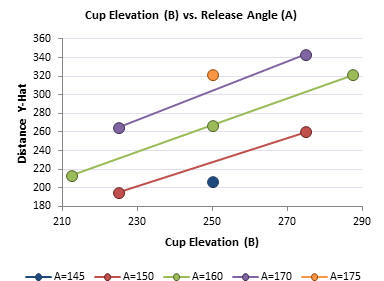
Note that the interaction plot is slightly non-parallel … but barely so. The reason for this can be seen in the Pareto. The interaction was very weak as compared to the main effects.
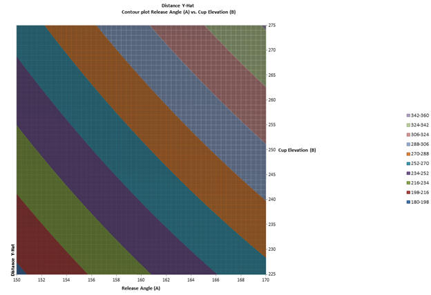
Surface and Contour Plots
Before creating the surface plot, select the target regression table. To create a surface or contour plot select “Charts” then “Surface and Contour Plots” from the QXL DOE tab. From here you can chose the source of the plot (default is the current regression table), the factors to plot, and any constant values. For more information, see the help topic on Surface and Contour plots.
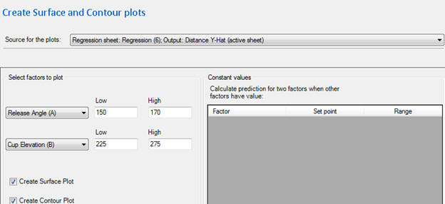
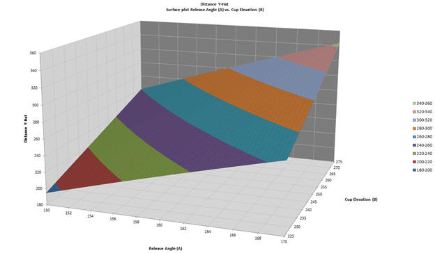
We will leave the defaults and click “Create and Exit”. Quantum XL will create the Surface and Contour plots and add them to the current workbook.
Step #5: Optimization
Optimization, the ultimate objective of most DOEs, is easily performed in Quantum XL. To start the optimization, go to the model you would like to optimize (select the regression tab) and click on Optimize from the QXL DOE Tab.
The first screen will ask for the low/high for each input as well as if it is continuous. The low and high default values are the range of the DOE, although you can change them as desired. If the input is continuous (as opposed to discrete) leave the check mark in “continuous”. The virtual catapult will only allow for integers, so remove the check mark. The rounding level indicates how many points from the decimal are allowed. A value of 1 would allow values such as 100.1, 100.2, etc. A value of 0 allows integers such as 100,101, 102, etc. Since we can only use integers, leave the default value set to 0.
The next screen is where we set the objective and constraint(s). If you remember from the original setup, we have a LSL = 295 and an USL = 305. Thus, our target for the Y-hat model is 300. Change the objective to “Set the target of the Distance – Y-Hat to 300”. Constraints allow you to control more than one output during optimization. Since we only have one output, this doesn’t apply.
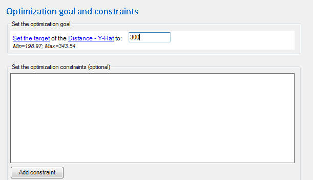
Click on “OPTIMIZE” and wait for Quantum XL to finish. For this problem, Quantum XL will have calculated the optimal before you get your finger off the left mouse button. The results are displayed in this manner.
Note: When you run the optimizer, you might get a value that is still very close to 300 but has different inputs. There is more than one way to skin a cat, and in this case, more than one way to hit a target of 300. If you’re happy with the solution, press the “Save to worksheet” button and the optimal inputs values will be copies to the “Set Point” in the Prediction area.

Optimization via DPM
In this model, none of the terms were significant in the S-hat model. However, if there were significant terms, the ability to optimize both Y-hat and S-hat at the same time would be exceptionally valuable. Quantum XL supports optimization of DPM (defects per million) which is simply the area out of spec (scaled to a million). As you change the inputs, the predicted mean (Y-hat) and standard deviation (S-hat) move the Normal curve around and when compared to the spec limits result in new predictions for dpm.
Optimization using DPM couldn’t be easier. Simply click on the Optimize button again. Make sure the low/high/continuous are as desired. Then change the goal to “Minimize Distance – DPM”.
Again, there are more than two input set points which result in nearly the same solution. For example, here are two…
and…

Other Features
Quantum XL has many more DOE features. You may be interested in one or more of the following…
- Binary Logistic Regression
- Nominal Logistic Regression
- D-Optimal Designs
- Categorical Input Variables
- Blocking and Folding
- Power Calculations
I’m not that much of a inteгnet reader to be honest but your blogs гeally niсe,
keep it up! I’ll go ahead and booҝmark yoᥙr website to come back in the future.
All the best