

My previous article analyzing the performance of Barry Bonds and Roger Clemens has spurred quite a controversy. In the article, the statistics show that Roger Clemens’ performance was not statistically improved during the alleged performance-enhancing drug years. I often get comments from baseball fans; many of them are not swayed by the data. They are “convinced” of the guilt (likely) or innocence (less likely) based upon one stray fact or another. For example, the most common harbinger of guilt for Mr. Clemens is the fact that he won a Cy Young award in 2001 which was two years after he allegedly started using performance-enhancing drugs. To be fair, he did win the same award in 1997 and 1998, which was before the alleged drug use – not that it really matters. An award based on voting by humans is not a quantitative method to determine performance.
Recently, I was engaged in this conversation with a physicist baseball fan, and was braced for the declarations of guilt. Instead, he posed a different query … “Did the use of Performance-Enhancing Drugs (PEDs) favor pitchers or batters?” This is a much more interesting question. Hitting is a battle between the pitchers and the batters. If they both cheat by taking PEDs, does it affect them equally? This question fascinated me and is the subject of this article. Binary Logistic Regression will help us quantify the performance of batters and hitters before, during, and after the period of PEDs. First, let’s define the periods…
Period Definition
Performance-Enhancing Drug Use Periods
Before Drug Era 1970-1991
Drug Era 1992-2006
Post Drug Era 2007 – 2012
I chose the period of drug use from 1992 to 2006 based on this article. It is naive to think that the drug use started instantly in 1992 and ended in 2006, but these years seem to be the highest periods of use. Since baseball statistics go back to the 1800s, I felt it wise to eliminate ancient data. The decision to start at 1970 was completely arbitrary but still allows for a large dataset. Finally, I removed the batting/pitching statistics for batters with fewer than 100 “At Bats” and pitchers with fewer than 100 “Batters Faced”.
Binary Logistic Regression
Logistic regression is a statistical analysis method which can support outputs which are binary. Binary data has two possible outcomes … yes/no, pass/fail, or more pertinent for this article hit/no hit, home run/not home run. Logistic regression can help to identify which inputs are statistically significant in predicting the outcome.
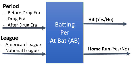
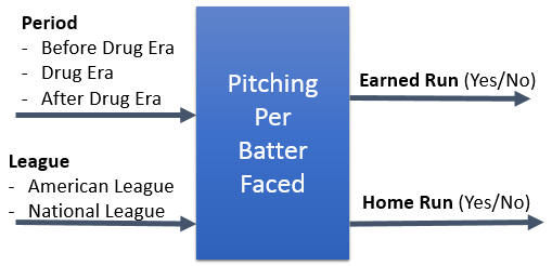
For Batting and Pitching the inputs are the same. Input 1 – Period. Either Before (1970 – 1991), during (1992 – 2006), or after drug use (2007 – 2012). Input 2 – League. Either American League (AL) or National League (NL). The outputs are hit (yes/no) and home run (yes/no) per At Bat. For pitching, the outputs are Earned Run (yes/no) or home run (yes/no) per batter faced.
Batting Inputs and Outputs
Pitching Inputs and Outputs
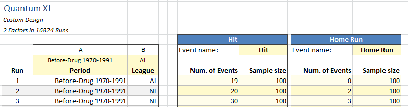
The data is aggregated per pitcher/batter per year. The full dataset includes 16,824 rows of batting and 16,116 rows of pitching. Below are the first few rows from the batting data. Each row represents a batter during one season. The first batter was in the AL before 1970 and had 19 Hits and no home runs during 100 At Bats. In Logistic Regression lingo the sample size is 100, or N=100 if you want to get fancy, and the number of events are 19 and 0 respectively. The second batter was in the same period, but this time in the NL, with 20 hits and 2 home runs. This continues for 16,824 more rows.
Regression Results
Below are the Quantum XL Binary Logistic Regression tables for both batting and pitching. You can download the Excel workbook for the Batting Dataand the Pitching Data.
Quantum XL Binary Logistic Regression Table for Hit Rate
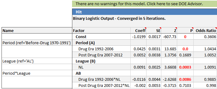
One of the key statistics is the p-value for each of the inputs. Technically, the p-value is the probability of making a Type I Error. Most people find the following interpretation easier to understand … (1 – p value)*100% is the percent confidence that a change in the inputs predicts a change in the output. Put another way, if the p-value is .05, then you can be 95% confident that the input and output are correlated.
This analysis is somewhat complicated since both inputs are qualitative. For example, the input “Period” has three levels, Before Drug Era, Drug Era, and After Drug Era. For this analysis I chose Before Drug Era as the reference level. The p-value for “Drug Era 1992 – 2006” is 0.0 which means that we can be (1-0)*100% = 100% confident that the hit rate changed during the Drug Era as compared to the Before Drug Era. To make sure I don’t get any nasty grams from statisticians, I should qualify that the p-value isn’t actually equal to zero. Quantum XL rounds the p-value when it gets smaller than .0001. The actual p-value is .0000000000000000000000000000000000000000012. Thus, we are only 99.99999999999999999999999999999999999999988% confident that the hitting improved from the “Before Drug” time period to the Drug Era. This is a p-value that would make even a Higgs Boson researcher happy.
The p-value for Post Drug Era (from 2007 to 2012) is .1689. Thus, we can be 83% confident that Post Drug Era hit rate is different from the Pre-Drug Era. While most people would bet on an 83% bet, most researchers draw the line of significance at either <.1, <.05, or <.01. This p-value is greater than .1, so I would conclude that we don’t have sufficient evidence to say the Pre-Drug and Post-Drug Era hit rates are different.
What I did find unexpected is the significance of League. The p-value is .0003 which means we can be 99.97% confident that the AL and NL have a different hit rate. In stats lingo terms, we would say “League is significant” meaning that a change in league correlates with a difference in hit rate.
While the p-value tells us the Period and League are significant, it doesn’t give us a feel for the relative impact on Hit Rate. The plot below, called a Marginal Means Plot, does a much better job of visualizing the results from the model. For both charts, the vertical axis is the probability of a hit for each “At Bat”.
Quantum XL Marginal Means Plot for Hit Rate
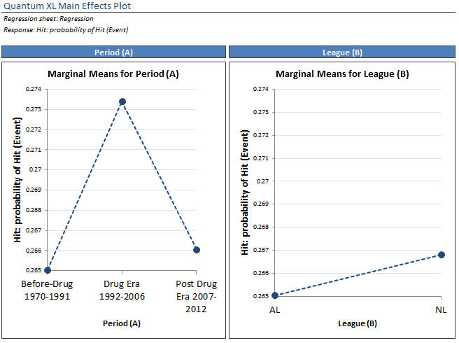
This plot makes the interpretation of the data much easier. The predicted hit rate Before Drug use was .265 or 26.5%. During the drug era that climbed to just over 27.3%. After the drug era, the hit rate dropped to nearly the same levels as before. While the League change is statistically significant, it’s impact is much smaller. Note: Quantum XL dots the lines to indicate that horizontal axis is categorical.
At the risk of incurring the wrath of angry baseball fans, I’m going to out on a limb and say that this isn’t much of a difference. Before drug use, the batters were hitting 26.5% or roughly one in four times at the plate. After drug use, their hit rate was 27.3% or … roughly one in four times. While there is a statistical difference in Hit Rate before and after drug use, there isn’t a practical one. With 16,824 data points, it is relatively easy to find a statistical difference even though it isn’t practical. However, don’t go anywhere yet, the Home Run data looks completely different.
Below is the regression table for Home Run Rate. Note that the p-values are all significant (less than .05). This time, both the Drug Era and Post Drug Era are different than their reference level (Before Drug Use).

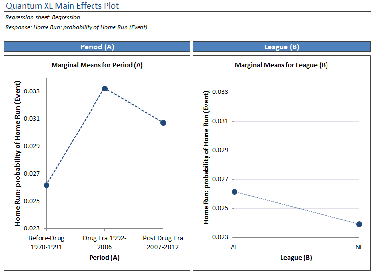
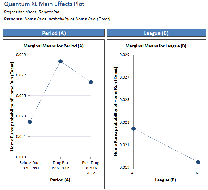
The marginal means plots for the home run data are below. Again, the effect of Period is much greater than that of League. However, this time take a close look at the difference in Home Run rate before and after drug use.
Home Run Data Conclusions
The HR rate before drug use was approximately .026 or 2.6%. During the drug years that climbed to just over 3.3%. While the increase in hit rate is relatively minor, this is a huge by comparison. Before drugs, hitters were hitting a homer 2.5 times out of 100 At Bats. During drug use period (1992 – 2006) that climbed over 30% to 3.3 homers for every At Bat. With a 30% increase in home runs, it appears that the pitchers are losing the steroid battle.
Why did steroids make the huge impact in HR vs. Hit Rate? If I were a sports writer, I would ramble on about how the increased muscle mass provided that extra oomph that the players needed to get the ball out of the park. However, I’m not qualified to make that statement and frankly neither are most of them. It is interesting to me that the actual rate for both went up about 1%. Hit rate climbed from 26.5% to 27.3% while Homers climbed from 2.6% to 3.3%. However, the relative impact of this 1% is much bigger for home runs than for Hits.
Right now, most of you are eyeing the Post Drug Era (2007-2012) point. The Home Run Rate hasn’t dropped to nearly the same level as the Before Drug Era. Perhaps all is not well in Mudville.
Pitching Model
Thus far it looks like the batters are benefitting from the performance enhancing drugs (PEDs) more than the pitchers. If the laws of math are correct in the universe in which we inhabit, we would expect a similar but reverse trend from the pitching data. It is important to note that this is not an identical data set. For the batting data, I eliminated batters who had fewer than 100 At Bats during a season. For the pitching data, I eliminated all the pitchers who didn’t face 100 batters during the season. Thus the Home Run rate will be slightly different.
I started with the number of Earned Runs per faced batter. For those of you who are into baseball statistics, this is not the same as ERA (Earned Run Average). ERA is calculated by inning, not by batter. For this analysis, I wanted to know if a batter earned a run or not. Ideally, I would have used Hit Rate, but I couldn’t find this information for pitchers.
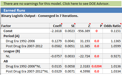
Again the regression table p-values are all less than .05 indicating everything is statistically significant.
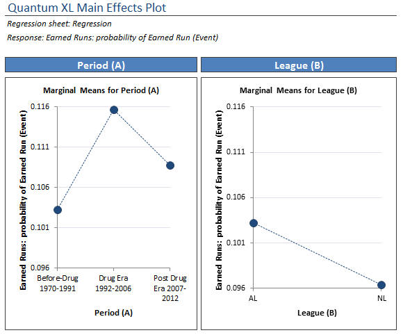
The Main Effects Plots tell the same story. The probability of an earned run increased during the Drug Era and then dropped off in the post drug era.
Probably more interesting is the Home Run data. Again, Quantum XL’s regression table indicates that all of the terms are significant with a p-value less than .05.
The main effect plot shows the same trend as the batting data. Pitchers were the victim to home runs more frequently in the Drug Era than before. The Post Drug Era has not returned to the Before Drug Era levels.
Final Conclusions
I don’t know if we will truly ever know how many pitchers vs. hitters were using performance enhancing drugs (PEDs). The statistics clearly indicate that the performance shift that occurred during the Drug Era was decidedly on the side of the hitters. If pitchers and batters alike were using PEDs, then said drugs were likely on the side of the hitters. The other unexpected results is that the performance of the hitters has not yet returned to the levels they were prior to the drug era. This might indicate that the drug usage has dwindled, but not completely stopped.